Recently I've been having some adventures with application tuning on GPUs. Unfortunately, the information available online on profiling them is scattered and sparse - so I wanted to give back and showcase some things I learned in this blog post. We'll look in-depth at some GPU concepts that are important to know when measuring GPU efficiency, and at Nsight Compute - an Nvidia tool for profiling a kernel running on a GPU.
For an example workload, we'll look at softmax - a staple component of deep learning and LLMs - and look at how we can use GPU profiling to significantly speed up a naive implementation.
0. What is softmax?
Before we really get started, let's go over the softmax function. Softmax is a way of normalizing vectors, transforming their inputs into probabilities that add up to and giving a larger weight to larger inputs.
Formally defined, if we mark softmax as , and we have a vector , then:
Some examples that get the point across:
Softmax is ubiquitous in deep learning and LLMs. It appears prominently in Google's infamous "Attention is All you Need" paper:
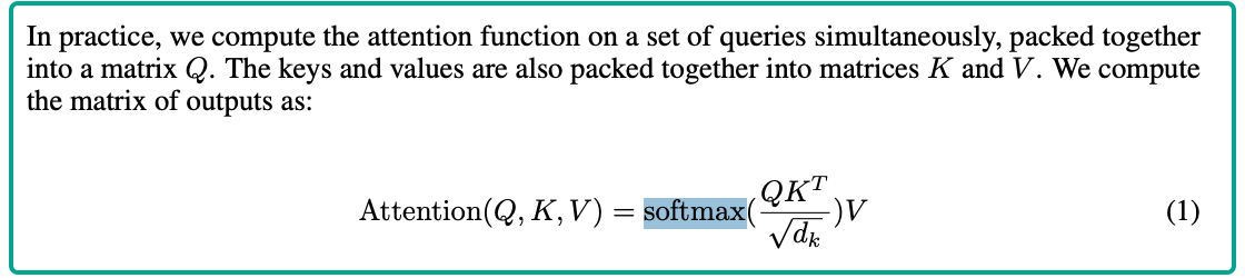
A core part of LLMs is calculating attention scores of tokens relative to each other. Softmax is used to normalize these scores, and in a typical LLM can be callled many thousands of times in a given inference run. Efficient softmax implementations are important for squeezing out LLM performance.
Throughout this blog post, we'll be running softmax on a two-dimensional array - our bottom-line goal is to get it to run as fast as possible.
We'll work with a matrix of shape , where each element is a 4-byte float32 - a total of 2000MiB per matrix.
1. Starting off with CPUs
Let's start off with a naive, single-threaded implementation on a CPU. Before we do, let's note something about the softmax equation: - it works with exponents. Exponents are tricky, because they get large very quickly and will overflow our 4-byte calculations. The common way of dealing with this is to first calculate:
And then subtract from the vector values, such that we calculate:
Fun Fact
This trick for ensuring numerical stability during softmax makes use of a useful softmax property. For any constant vector :
With that in mind, this is our naive implementation on a CPU:
import numpy as np, time

def softmax_np(x):
    x = x - x.max(axis=-1, keepdims=True)
    exp_x = np.exp(x, dtype=np.float32)
    return exp_x / exp_x.sum(axis=-1, keepdims=True)

x = np.random.randn(32000, 16384).astype(np.float32)
REPEAT = 50

print("Beginning measurement:")

t0 = time.time()
for _ in range(REPEAT):
    y = softmax_np(x)
total_time = time.time() - t0
print(f"Total: {total_time:.3f}s")
print(f"Average per iteration: {total_time / REPEAT:.6f}s")
Running the script on a c7g.12xlarge shows an average of 2.71 seconds/iteration. Our naive implementation
makes use of a single core - we're not making full use of our c7g.12xlarge's 48 vCPUs. PyTorch's softmax implementation
uses all available vCPUs, so we'll see how long it takes if we use that non-naive implementation:
import torch, time

x = torch.randn(32000, 16384, dtype=torch.float32)
REPEAT = 50
softmax = torch.nn.Softmax(dim=-1)

print("Beginning measurement:")

t0 = time.time()
for _ in range(REPEAT):
    y = softmax(x)
total_time = time.time() - t0
print(f"Total: {total_time:.3f}s")
print(f"Average per iteration: {total_time / REPEAT:.6f}s")
And we can observe a more than 10x speed-up, to an average of 0.22 seconds/iteration. If going from one core to 48 cores gives us a 10x speed-up, how much of a speed-up can we get from the several thousands of cores in a GPU? Let's find out:
2. Naive implementation on a GPU
We're going to work in Google Colab, working in a Tesla T4 GPU runtime notebook.
Tip
Google Colab is one of those "I can't believe it's not butter free" products. To set up the notebook for GPU profiling, I ran this cell:
%%shell
wget https://developer.nvidia.com/downloads/assets/tools/secure/nsight-systems/2025_3/NsightSystems-linux-cli-public-2025.3.1.90-3582212.deb
dpkg -i NsightSystems-linux-cli-public-2025.3.1.90-3582212.deb
And then for every CUDA program I wrote, I ran these two cells:
%%writefile program.cu
<FILE CONTENTS>
%%shell
nvcc -arch=sm_75 program.cu -o program
# Running the program
./program
# Profiling the program
ncu --set full -o program_performance_report -f ./programAnd then downloaded the output program_performance_report.ncu-rep for analysis in Nvidia Nsight Compute.
Let's start off with a naive implementation. A quick recap for the uninitiated - our goal is to launch many thousands of threads on the GPU such that they compute softmax. These threads will be organized into a grid of blocks - each block is a grouping of threads.
Info
When we launch a CUDA kernel, we provide three parameters - the dimensions of the grid (i.e. the structure of the blocks), the dimensions of each block (i.e. the structure of the threads), and the number of bytes of shared memory dynamically allocated to each block in the kernel.
kernel<<<dimGrid, dimBlock, sharedMemorySize>>>(...);The first two parameters are of type dim3 - i.e. they have three dimensions. dimGrid.x can range from to , and
dimGrid.y, dimGrid.z can both range from to - for a maximum of almost blocks.
The number of threads per block is far more restrictive - a maximum of 1024 threads. No limits on block dimensions exist, so long as this limit is met.
Let's write a straightforward kernel - each block will work on an entire row, and we'll split each block into 256 threads that work together.
constexpr int ROWS = 32000;
constexpr int COLS = 16384;
constexpr int THREADS = 256;

__global__ void softmax_kernel(const float* __restrict__ in,
                                     float*       __restrict__ out,
                                     int cols)
{
    extern __shared__ float shmem[];
    int row = blockIdx.x;
    int tid = threadIdx.x;
    const int stride = blockDim.x;

    // Calculate the max for each thread's elements
    // Thread 0 indices -> [0, 256, 512, ...]
    // Thread 1 indices -> [1, 257, 513, ...]
    float local_max = -FLT_MAX;
    for (int c = tid; c < cols; c += stride)
        local_max = fmaxf(local_max, in[row * cols + c]);
    shmem[tid] = local_max;
    __syncthreads();

    // Reduce max between all threads
    for (int off = stride >> 1; off; off >>= 1) {
        if (tid < off) shmem[tid] = fmaxf(shmem[tid], shmem[tid + off]);
        __syncthreads();
    }
    float row_max = shmem[0];

    // Calculate (e^{x - max}) for every element in the row
    float local_sum = 0.0f;
    for (int c = tid; c < cols; c += stride) {
        float e = expf(in[row * cols + c] - row_max);
        out[row * cols + c] = e;

        // Keep track of the sum of the row's elements as we go
        local_sum += e;
    }
    shmem[tid] = local_sum;
    __syncthreads();

    // Combine the sum of all threads for the total sum of the row
    for (int off = stride >> 1; off; off >>= 1) {
        if (tid < off) shmem[tid] += shmem[tid + off];
        __syncthreads();
    }
    float row_sum = shmem[0];

    // Finally, divide (e^{x - max}) by the sum of the row for the final result
    for (int c = tid; c < cols; c += stride)
        out[row * cols + c] /= row_sum;
}

int main() {
    ...
    dim3 grid(ROWS);
    dim3 block(THREADS);
    size_t shmem_bytes = THREADS * sizeof(float);
    softmax_kernel<<<grid, block, shmem_bytes>>>(d_in, d_out, COLS);
    ...
}
We can run this and observe that it takes an average of 0.043 seconds/iteration - a further 5x speed-up on our vCPU-saturating attempt, and a full 50x speed-up over our initial naive solution!
But can we do better (spoiler: Yes)? Let's download the profiling report and open it up in Nsight Compute.
3. Profiling our naive implementation
We'll open up our profiling .ncu-rep file in Nsight Compute and get to work.
Some things immediately pop up:
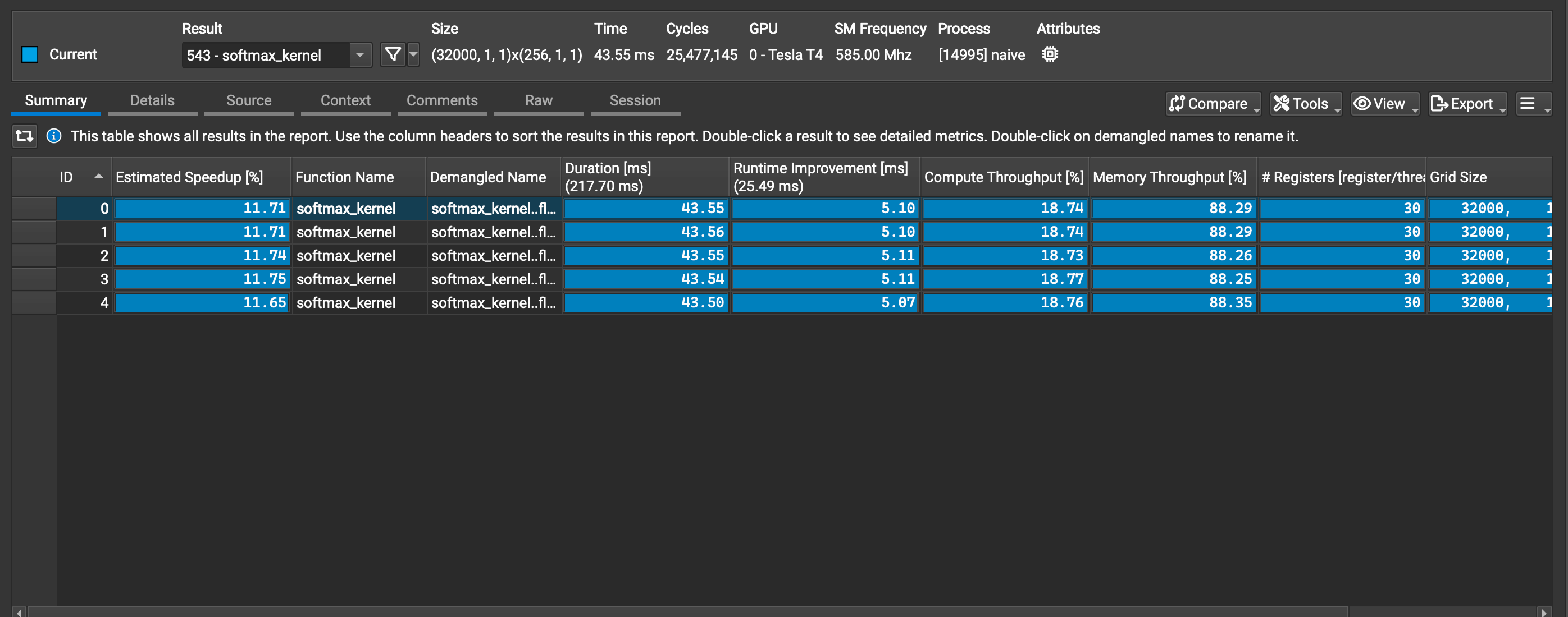
- I ran the kernel five times to get an average runtime - we see each of these five runs profiled separately.
- In the topbar, we see basic information on; 32,000 blocks, 256 threads per block, the GPU we're running on and its frequency. Note that the number of cycles is a reflection of .
- We see a very low compute throughput of just 18.74%, but a relatively high memory throughput of 88.29%, suggesting that we're limited by memory in this kernel.
The real goodies are to be found in the "Details" tab. There's a lot of noise in there, so we'll focus on the sections that are most relevant to us - "GPU Speed of Light Throughput", "Scheduler Statistics", "Warp State Statistics", "Memory Workload Analysis", and "Compute Workload Analysis." Each of these sheds some light and together they'll illuminate a full picture.
3.1 GPU Speed of Light Throughput
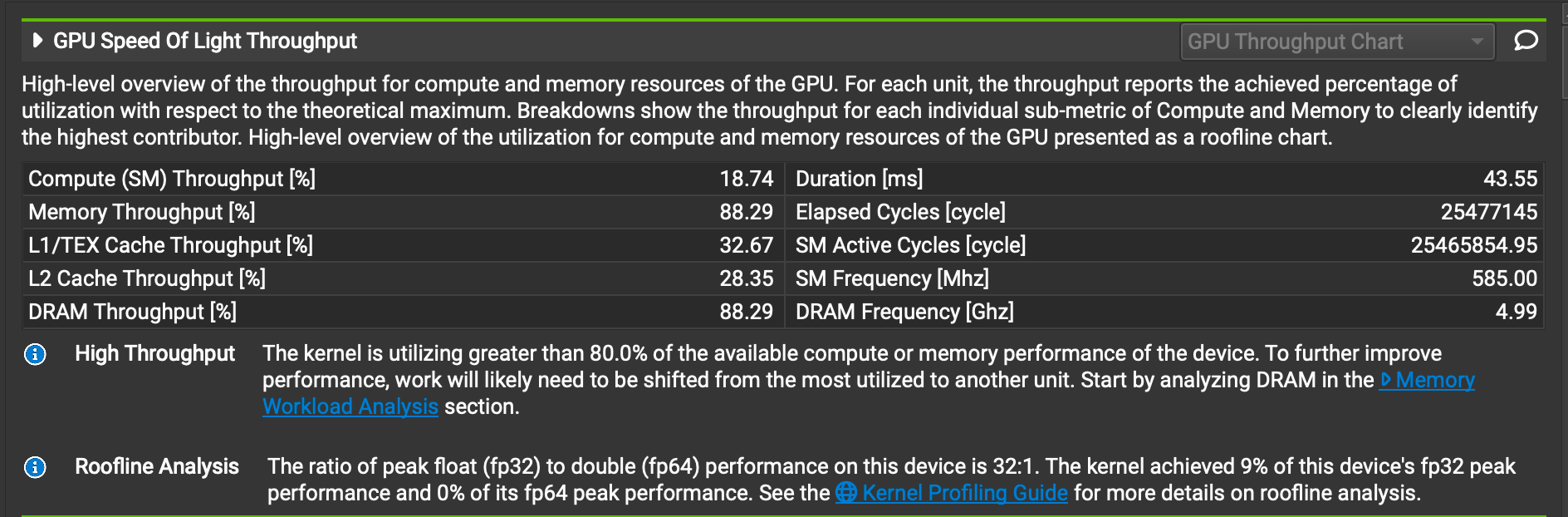
There are a few data points here that show poor cache utilization, and poor "fp32 peak performance." We also again see our compute and memory throughput figures.
It's hard to know definitively at this point, but all of the data points in this section suggest that we're not doing enough work with the data we're reading from memory. If we can find a way to "do more" with the data being read, most of these numbers should improve.
3.2 Scheduler Statistics and Warp State Statistics
Before we look at the profiled scheduler statistics, let's review some Nvidia GPU scheduling basics. This is a bit in-depth, so if you're already familiar or just want to get to the profiling, feel free to skip ahead to the image below.
We saw in a previous note that we can launch up to almost blocks - obviously no GPU has anywhere near the capacity for running that many blocks simultaneously, so there are a few details that are worth knowing when it comes to how these blocks are scheduled.
GPUs can be visualized as "lots and lots and lots of cores." But there are two layers that group these hardware cores:
-
The first layer is an architectural one - Nvidia GPUs are split into streaming multiprocessors, or SMs, with each SM being composed of many cores. For instance, the Tesla T4 GPU has 40 SMs, with 64 cores per SM, for a total of 2560 cores. Importantly, when a block is scheduled, it is scheduled on a single SM; an alternative way of looking at this is that all threads in a block execute on the same SM. Since many blocks can be assigned to an SM, and an SM has finite resources - it is up to the GPU's scheduler to intelligently execute multiple blocks in parallel on a given SM.
-
The second layer is an implementation detail - how are multiple threads within the same block scheduled on an SM? Enter the warp - a unit of 32 threads from the same block. It is the most granular unit of scheduling on a GPU - blocks are broken down into warps, and these warps are then scheduled on SMs. If we zoom into a single warp, during a given cycle, all threads in the warp are executing the exact same instruction. This raises some obvious questions regarding branch handling and thread divergence, but we won't get into that right now.
Fun Fact
How do warps actually work? The hardware cores in each SM are broken down into processing blocks, and each processing block shares a common instruction fetch/dispatch unit. That's a pretty cool contrast with CPU cores, where each core needs its own instruction fetching - a small example of how GPUs can accomplish more with less.
Now, we need to understand how the GPU runtime juggles warps in an SM. Each SM has model-specific limitations across two dimensions - 1) the number of blocks schedulable on the SM, and 2) the number of warps schedulable on the SM.
This has subtle implications. The T4 supports up to a total of 16 blocks on each SM, and a total of up to 32 warps (1024 threads) per SM. Now, if we try to assign 16 blocks, each with 32 threads - they'll all get scheduled successfully on the SM, and we'll end up with an occupancy of 100%. But, if we launch those 16 blocks with 16 threads each - we'll end up with an occupancy of only 50%, and because of the blocks limitation we will not be able to schedule any more blocks! As another example, if we have a block of 768 threads, we'll only be able to launch one block without overflowing the threads limitation, for a total of 768 threads on the SM - an occupancy of 75%. A lower occupancy can quickly lead to degraded performance when the scheduler finds itself lacking available warps for execution.
And there's yet another source of potential inefficiencies. As opposed to CPUs, GPUs support zero-overhead scheduling - one thread can be swapped with another with far less overhead than on a CPU. This is accomplished by giving each SM substantially more registers than available in a CPU core - in the T4 we have 65536 registers per SM! But this means that if the SM is 100% occupied then all threads should use no more than an average of 64 registers - otherwise there won't be enough to go around. And if the threads need more registers to go around than are available, then they'll be spilled over to memory, impacting performance.
So we're now aware of two significant limitations as it relates to maximizing our usage of our GPU - making sure that we're writing our program in a way that ensures maximum occupancy of each SM, and making sure that we're not consuming more registers than available in an SM. Moreover, we know that if a warp ends up waiting on anything - e.g. memory access - and there's not another warp to take its place, that signifies 32 cores that are just hanging around not working. With this in mind, let's look at our "Scheduler Statistics."
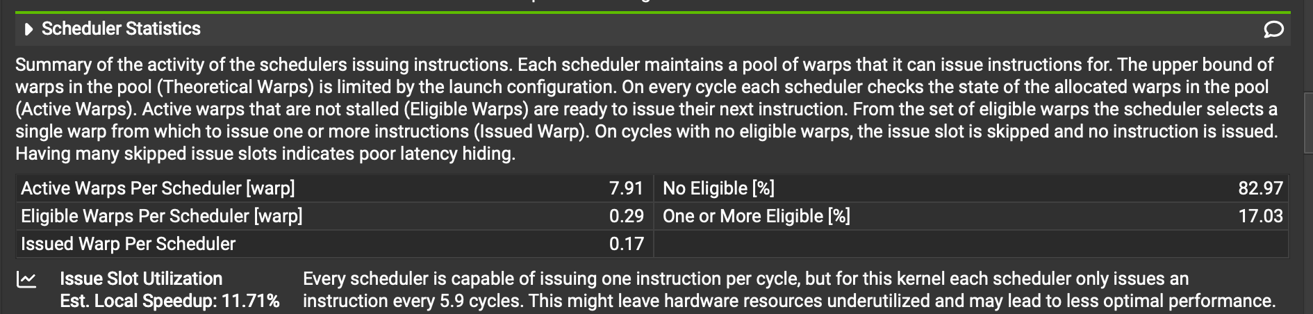
These numbers aren't great. There's a bottom-line summary for us: "Every scheduler is capable of issuing one instruction per cycle, but for this kernel each scheduler only issues an instruction every 5.9 cycles." In other words, more than 80% of execution opportunities aren't being used. There's an average of 7.91 active warps - i.e. warps that will eventually need to run - per scheduler at any given time, but only 0.29 are able to run. In other words, more than 90% of our warps are sitting around waiting for something, leading to many unutilized cores.
Moving on to "Warp State Statistics":
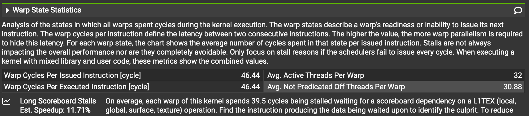
The right two numbers are great - 32 active threads per warp is the maximum number possible, and 30.88 "Avg. Not Predicated Off Threads Per Warp" just means that almost all 32 threads are executing "real instructions" and not disabled due to branch divergence, close to the maximum 32 possible.
But the left two numbers aren't great - we're only issuing one instruction every 46.44 cycles when we should be issuing much more frequently. And we can see that of those 46, a full 39.5 are spent waiting for a "scoreboard dependency" - i.e. waiting for a register to resolve with data from a memory load.
These two sections start to flesh out the intuition we've started to develop in the previous section - our problem is inefficient memory access.
3.3. Compute & Memory Workload Analysis
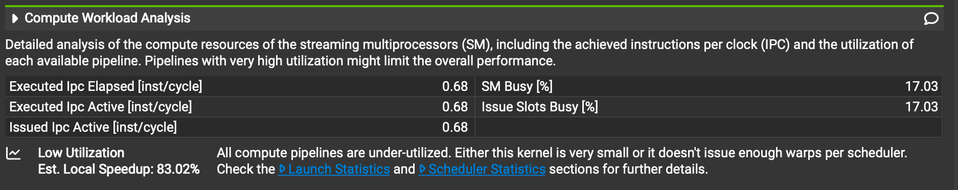
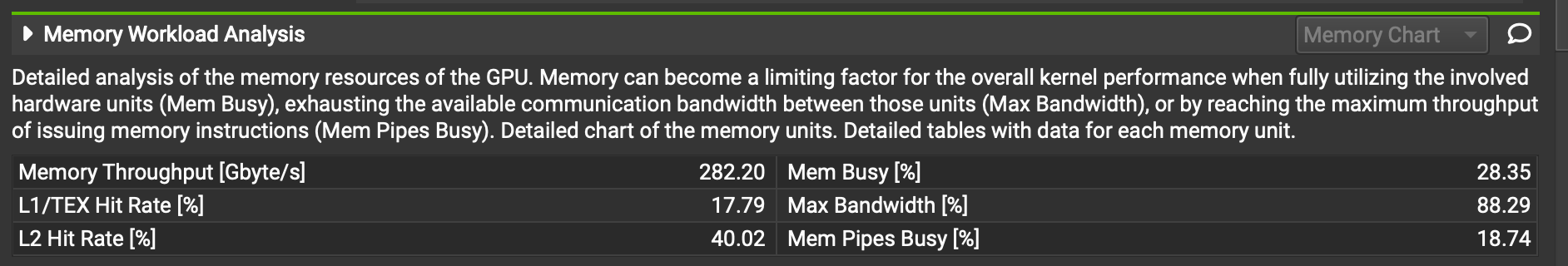
We can see that our SMs are only active 17.03% of the time and that all compute pipelines are underutilized.
Moreover, only 18% of memory accesses are L1 cache hits - this ties back to the 39.5 cycles of scoreboard stalling we saw earlier.
These numbers provide the final proof for our bottom-line conclusion - we're not doing enough with the data we're retrieving.
3.4 Initial Profiling Summary
These numbers help us verify that our program is written in a memory-inefficient way. We have lots of compute capacity, but we're not making full use of it - most of our kernel's time is spent waiting for memory access, and we've written our memory access in a cache-unfriendly way.
We need to relook at our program to fetch memory in a more intelligent way - we'll try to ensure that it's cache-friendly, and that we do as much work as possible with every byte we fetch.
3.5 Source Code Analysis
You might have noticed something pretty cool - all of this profiling hasn't looked at the source code at all. In fact, the compile command mentioned above:
nvcc -arch=sm_75 program.cu -o programDoesn't compile the program with source information. For that, we need:
nvcc -arch=sm_75 naive.cu -o naive -G -gWhen we open up the profiling of this new binary, we can look at the "Source" tab to see the performance profile of each line in the source. Some lines that are especially pertinent to our conclusions are:


These three lines are responsible for a cumulative 68% of warp stalls. They read from global memory, continuously stalling on that memory access.
4. Optimizing our program
Informed by our profiling, we'll rewrite our program to tackle some inefficiencies. In the original kernel, we fetched from in twice.
This time, we'll keep the initially read values in a local array, so they can be reused.
We'll also refrain from writing to out twice - we'll write to it just once.
constexpr int ROWS = 32000;
constexpr int COLS = 16384;
constexpr int THREADS = 1024;               // Changed from 256
constexpr int ITEMS   = COLS / THREADS;     // 16 elements per thread

__global__ void softmax_kernel(const float* __restrict__ in,
                                     float*       __restrict__ out,
                                     int cols)
{
    extern __shared__ float shmem[];
    int row = blockIdx.x;
    int tid = threadIdx.x;
    const int stride = blockDim.x;

    // New - thread-local cache for data read from memory
    float thread_elements[ITEMS];

    // Calculate the max for each thread's elements, and load the elements into a local array
    float local_max = -FLT_MAX;
    for (int i = 0; i < ITEMS; ++i) {
        int col             = tid + i * stride;
        float x             = in[row * cols + col];
        thread_elements[i]  = x;
        local_max           = fmaxf(local_max, x);
    }

    shmem[tid] = local_max;
    __syncthreads();

    // Reduce max between all threads
    for (int off = stride >> 1; off; off >>= 1) {
        if (tid < off) shmem[tid] = fmaxf(shmem[tid], shmem[tid + off]);
        __syncthreads();
    }
    float row_max = shmem[0];

    // Calculate (e^{x - max}) for every element in the row
    float local_sum = 0.0f;
    for (int i = 0; i < ITEMS; ++i) {
        thread_elements[i] = expf(thread_elements[i] - row_max);
        local_sum += thread_elements[i];
    }

    shmem[tid] = local_sum;
    __syncthreads();

    // Combine the sum of all threads for the total sum of the row
    for (int off = stride >> 1; off; off >>= 1) {
        if (tid < off) shmem[tid] += shmem[tid + off];
        __syncthreads();
    }
    float row_sum = shmem[0];

    // Finally, divide (e^{x - max}) by the sum of the row for the final result
    for (int i = 0; i < ITEMS; ++i) {
        int col = tid + i * stride;
        out[row * cols + col] = thread_elements[i] / row_sum;
    }
}

int main() {
    ...
    dim3 grid(ROWS);
    dim3 block(THREADS);
    size_t shmem_bytes = THREADS * sizeof(float);
    softmax_kernel<<<grid, block, shmem_bytes>>>(d_in, d_out, COLS);
    ...
}
This only slightly modified kernel runs in 0.017 seconds/iteration - more than twice as fast as the previous kernel! If we open up its profiling in Nsight Compute, we see these changes:
- Memory throughput: 88.29% -> 84.76%. We still make close-to-saturated use of memory bandwidth.
- Compute throughput: 18.74% -> 48.00%. We've almost tripled our usage of the GPU's compute resources!
- SM Busy: 17.03% -> 41.76%. Similar to the previous metrics, we observe significantly increased saturation of the GPU's compute resources.
- L1 Hit Rate: 17.79% -> 0.00%. This is not a degradation! It's actually proof that we're making improved use of data we're loading. We have no cache hits because every cache line we bring in is fully consumed, we don't need to refetch any of its data.
- Eligible Warps per Scheduler: 0.29 -> 1.63. This means that far more warps are available for execution per scheduler - fewer are stalling on memory access.
- Warp Cycles Per Issued Instruction 46.44 -> 18.98. Warp instructions execute far faster, waiting for far fewer cycles for memory access.
5. Additional optimizations
There are a few additional optimizations we could do here, but they'll have a less dramatic impact. One really cool one is warp-level reduction - in our previous two kernels, we calculated the max and the sum of each row through continuous reduction across all threads in a block. This is done using shared memory, which is fast enough - but warp-level reductions don't go through memory at all! They make use of clever hardware functionality for reducing the data for each warp - drastically cutting down the shared memory we need for the reduction.
But at this point, we'll have diminished returns from just straight optimizations - we'll need to start looking at algorithmic optimizations, i.e. a deeper look at how we calculate softmax itself. There are algorithmic changes to softmax that enable us to only loop over the row twice, instead of thrice as we currently do (once for max, once for sum, once for final calculation) - but Nsight Compute isn't of much value here, so we'll leave that for another day.
6. Conclusions
We started with a naive CPU implementation that took 2.71 seconds/iteration, and ended with a 0.017 seconds/iteration implementation. Along the way we covered some of the fundamentals of GPU performance considerations, and learned how to work with Nsight Compute.
Here's a final rundown of our performance:
| Version | Average Time/Iteration | Speed-up |
|---|---|---|
| CPU Naive | 2.71 seconds | 1x |
| Pytorch Softmax (48 vCPU) | 0.22 seconds | 12x |
| GPU Naive | 0.043 seconds | 63x |
| GPU Optimized | 0.017 seconds | 159x |
We've only covered the tip of the iceberg of GPU profiling and optimization. We only focused on CUDA kernel-level optimization, using Nvidia's Nsight Compute, but most applications need to look at system-level profiling, showing the interplay between CPUs, GPUs, the operating system, etc. Nsight Systems is Nvidia's tool for this. There's a whole world of GPU optimization techniques that we didn't cover in our simple example.
With the ever-increasing appetite for heavy computations on GPUs (including what must be billions of softmax computations performed hourly across the planet!), GPU programming and profiling is increasingly useful - and also immensely fun. Hope you enjoyed!